goMortgage Tutorial
Table of Contents
Preparations
So, you want to build a mortgage model. Where do you start? Well, having some loan-level data is a necessity. I suggest you start with the Fannie Mae data. It’s free and extensive, going back to January 2000. There are two data sets: their “standard” dataset of fixed-rate loans and a dataset of exclusions that includes ARMS and loans with non-standard underwriting. I have an app to import this into ClickHouse and good news! – goMortgage is already set up to handle the table. Even if your ultimate goal is to use goMortgage on different data, this is the easiest way to test drive it.
There is one other table you’ll need – a table of non-loan data. This table has fields for house prices, unemployment, income, labor growth rates and more. The data is monthly at a zip/zip3 level. The assemble package will produce the table you need.
OK, let’s suppose you have these two tables. What next? All of goMortgage’s activity is driven by a specification (*.gom) file. Let’s look through one of these.
The .gom file
The .gom entries are in a key/val format. Both the keys and values are case-sensitive. We’ll go through the file dq.gom This .gom file builds a delinquency model. It’s a hazard model, or perhaps better termed, a conditional softmax model. The model estimates the probability the loan is in one of 13 delinquency states each month of the forecast period. The forecast period is 180 months. The 13 delinquency states are: current, 1 through 11 months delinquent and 12+ months delinquent. The condition of “conditional” softmax is that (a) the loan exists at the beginning of the month and (b) it doesn’t prepay/default that month.
Let’s review the entries. The first key is the title which will appear on graphs. The next entry, “outDir”, is the one key that is always required. It specifies the location of the output of the run. When goMortgages runs dq.gom, all the non-ClickHouse output will be sent to “/home/will/goMortgage/dq”. The directory structure is here.
The next three keys instruct goMortgage to build the data it needs from source tables, then build and assess the model.
title: DQ model
outDir: /home/will/goMortgage/dq
buildData: yes
buildModel: yes
assessModel: yes
buildData
See here for details on buildData keys.
The code below specifies the data build. The loan-level data is sampled in two passes. See data build for details. The two blocks specify the target sample size, strata and where clauses for each pass. The where clauses restrict the choice set.
The pass 1 sampling is along the fields state, aoDt (as-of date) aoAge (loan age at as-of date) and aoDqCap6. aoDqCap6 is the as-of delinquency capped at 6 months (values greater than 6 are set to 6). goMortgage will do its best to stratify along these fields jointly, targeting an output data set of 30,000,000 rows. Each row is a loan at a specified (state, aoDt, aoAge, aoDqCap6). Of course, state is fixed for a loan and each loan has but one aoAge and aoDqCap6 at a given aoDt. The where1 clause specifies which loans are considered for the sample. The code essentially restricts the selection to loans that are active and less than 25 months delinquent.
The pass 1 sample is a compact representation. What we’re sampling in pass 2 is each loan in pass 1 at every possible month after aoDt (to determine the target date). The code directs the pass 2 sample to stratify along fcstMonth and trgDt targeting a sample size of 3,000,000. fcstMonth is the number of months since aoDt and trgDt is the target date. The where2 clause restricts the candidate set to dates that are after the as-of date and which are still active.
Note: you can specify the stratification field as “noGroups” if you want a simple random sample.
// fields to stratify on at pass 1
strats1: state, aoDt, aoAge, aoDqCap6
// target # of rows in output of pass 1
sampleSize1: 30000000
// at the as-of date, we restrict to active loans with a max dq of 24 months and balance greater than $10k
where1: aoAge >= 0 AND aoDq >= 0 AND aoDq <= 24 AND aoUpb > 10000 AND mon.zb='00'

// fields to stratify on at pass 2
strats2: fcstMonth, trgDt
// target # of rows in output of pass 2
sampleSize2: 3000000
// at the target date, we restrict to dates after the as-of date which are active.
where2:  trgZb='00' AND fcstMonth > 0
These keys specify the source and type of the input data. The “mtgFields” key specifies that this is Fannie data. The “econ” entries specify the ClickHouse table with non-loan data and the field to join on. The most granular geo field in the Fannie data is the 3-digit zip.
// fannie mortgage data created by https://pkg.go.dev/github.com/invertedv/fannie
mtgDb: mtg.fannie

// keyword specifies the source of the data
mtgFields: fannie

// non-loan data created by https://pkg.go.dev/github.com/invertedv/assemble
econDb: econGo.final

// the fannie data specifies geo location at a zip3 level
econFields: zip3
And, finally, these keys specify the location of the output. The “outTable” is the final output table of the process that goMortgage will use to build and assess the model. The table will be ordered by “lnId” (loan ID).
// outputs
pass1Strat: tmp.stratDq1
pass1Sample: tmp.sampleDq1
pass2Strat: tmp.stratDq2
pass2Sample: tmp.sampleDq2
// final table
outTable: tmp.modelDq
// key for final table
tableKey: lnId
buildModel
The sections below controls the model build. See here for details on buildModel keys.
The section below defines the model. The target of the model fit is the field “targetDq”. This field is not in the fannie table but calculated from the delinquency field – capping that field at 12. The target type is ‘cat’ since we want to estimate the probability of a loan being at each delinquency level.
The “cat” entry lists the one-hot features in the model. The “cts” entry lists the continuous fields. Note: goMortgage will normalize the continuous fields. The “emb” entry lists the embedded features. Each feature name is followed by the embedding dimension in braces.
The “layer
// targetDq is an int32 field that takes on values 0,..,13.
target: targetDq
// We treat targetDq as categorical - which will build a model with a softmax output layer
targetType: cat

// one-hot features.  Note, it's fine for this to take up multple lines
cat: purpose, propType, occ, amType, standard, nsDoc, nsUw, coBorr, hasSecond, aoPrior30, aoPrior60,
  aoPrior90p, harp, aoMod, aoBap, channel, covid, trgFcType, potentialDqMax, potentialDqMin

// Continuous features.  Note, these will automatically be normalized.
cts: fico, aoAge, term, y20PropVal, units, dti, trgUnempRate, trgEltv,
  trgRefiIncentive, lbrGrowth, spread

// Embedded features.  The embedding dimension is in the braces.
emb:  aoDq{5}; state {4}; fcstMonth{2}; trgAge{2}

// this is the model we're fitting.
layer1: FC(size:40, activation:relu)
layer2: FC(size:20, activation:relu)
layer3: FC(size:10, activation:relu)
layer4: FC(size:13, activation:softmax)
The next section controls the model building process. “batchSize” and “epochs” set what you think they do. The “earlyStopping: 40” ends the fit if the cross entropy calculated on the validation data fails to decline for 40 epochs. The learning rate entries specify the learning rate at the first and last (2000, in this case) epoch. The learning rate declines linearly.
// Other specifications for the model build.
batchSize: 5000
epochs: 2000
earlyStopping: 40
learningRateStart: .0003
learningRateEnd: .0001
The section below pulls the data. goMortgage consumes 3 datasets:
- model. This is the data used to fit the model coefficients.
- validation. This is the data used to determine early stopping.
- assessment. This is the data used to assess the model after it is fit.
The ‘modelQuery’, ‘validateQuery’ and ‘assessQuery’ entries specify the SQL to pull these.
A feature of the fannie app is that it creates a field “bucket” that assigns each loan an integer value 0 through 19. This value is sticky – a loan will always get the same value. Further, it is uncorrelated with other fields. This enables us ensure the three datasets consist of disjoint loans.
Finally, the queries have a placeholder “%s” instead of an explicit field list. goMortgage replaces this with the fields needed for the run.
// This query pulls the data for fitting the coefficients.  The %s will be replaced with the fields we need.
// The bucket field is a hash of the loan number.
modelQuery: SELECT %s FROM tmp.modelDq WHERE bucket < 10

// This query pulls the data for determining early stopping.
validateQuery: SELECT %s FROM tmp.modelDq WHERE bucket in (10,11,12,13,14)
assessModel
See here for details on assessModel keys. In the code below, the assessQuery pulls the data for the assessment.
You can save the assess data–augmented with the model output–back to ClickHouse. The ‘saveTableTargets’ give the field name followed by the columns of the softmax to sum to create it.
The last two entries, “addlCats” and “addlKeep”, keep additional fields that have not yet been specified. “addlCats” keep fields are internally created as one-hot fields. This can be necessary if you want to treat the field as categorical for assessment. The “addlKeep” fields are kept as-is internally. You may wish to keep fields for output to the SaveTable. For instance, lnId (loan ID) would never be used in the model/assess process, but you definitely want that in the output table.
assessQuery: SELECT %s FROM tmp.DqModel WHERE bucket in (15,16,17,18,19)

// save Assess Data + model output.
// The table will consist of all the fields used during the run plus any set of model outputs you specify.
saveTable: tmp.outDq

// We're saving five fields from the model output.
saveTableTargets: d120p{4,5,6,7,8,9,10,11,12}; d90{3}; d60{2}; d30{1}; current{0}

// Features not in the model we wish to keep and treat as categorical.  These can be used in the assessment.
addlCats: targetAssist, aoMaxDq12, vintage, aoDqCap6, numBorr

// Features to keep, either for assessment or to add to the output table.
addlKeep: lnId, aoDt, trgDt
goMortgage will automatically run the assessment on the features in the model. You may wish to run it on additional fields. These are supplied in the “assessAddl” key, below. The name,
// Additional fields for the assessment.
assessAddl: aoIncome50, aoEItb50,  trgPti10, trgPti90, ltv, aoMaxDq12, trgUpbExp, aoIncome90, msaLoc,
  aoPropVal, trgPropVal, vintage
The entries below specify an assessment. “DQ 4+ Months”, will appear on all graphs. Note that each entry ends in “aoDq”. This arbitrary value ensures these specs get grouped together. The assessment is conducted on the sum of the columns 4 through 12 of the softmax output - which corresponds to 4+ months delinquent. The assessment is sliced on the field aoDqCap6. That is, it will be done separately for each of the aoDqCap6 values (0 through 6).
// Run a by-feature assessment that is sliced by aoDqCap6 on the binary output that coalesces targetDq into two groups
// of (0,1,2,3) and (4,5,6,7,8,9,10,11,12).  aoDqCap6 is the delinquency status at the as-of date where the
// delinquency levels are 0 trough 5 and 6+ months.
assessNameaoDq: DQ 4+ Months
assessTargetaoDq: 4,5,6,7,8,9,10,11,12
assessSliceraoDq: aoDqCap6
Here’s another entry that slices by the field occ.
// Run another assessment that is sliced by occupancy.
assessNameOcc: DQ 4+ Months
assessTargetOcc: 4,5,6,7,8,9,10,11,12
assessSlicerOcc: occ
Note: specify “noGroups” as the slicer if you don’t want to slice by anything.
For a categorical target, goMortgage will produce KS and Decile plots, overall and for each level of the slicer. Further, it will produce Segment plots for each feature in the model and each field specified in “assessAddl”. For each feature in the model, goMortgage will also construct marginal plots.
Another form of assessment are curves. These will plot the model output and actual value averaged by the given field. Below, the DQ 4+ months values are averaged over the target year/quarter (trgYrQtr is a field in the table created by goMortgage).
// Run a by-curve assessment where the metric on the binary output that coalesces into two groups:
// 0-3 months DQ and 4+ months DQ. The graph will be two curves: model and average rate of 4+ months DQ
// where the average is over the distinct levels of trgYrQtr.
// trgYrQtr is the the Year & Quarter of the target date.
curvesNameyrQtrD120: Target Quarter, DQ 4+ Months
curvesTargetyrQtrD120: 4,5,6,7,8,9,10,11,12
curvesSliceryrQtrD120: trgYrQtr
As before, each key has appended a key “yrQtrD120” so that goMortgage knows these go together.
Finally, there are a couple of general settings:
// general
show: no
plotHeight: 1200
plotWidth: 1600
If “show” is set to “yes”, then each graph will also be displayed in your browser. This is usually a lot of graphs! “plotHeight” and “plotWidth” specify the plot dimensions, in pixels. The graphs are also written to files.
Output
(Click graphs to enlarge/reduce)
Curve Assessments
All these assessments are constructed using loans that were not part of the model build/validation early stopping. The graph below is the curve assessment described above. This model is very faithful to the data.

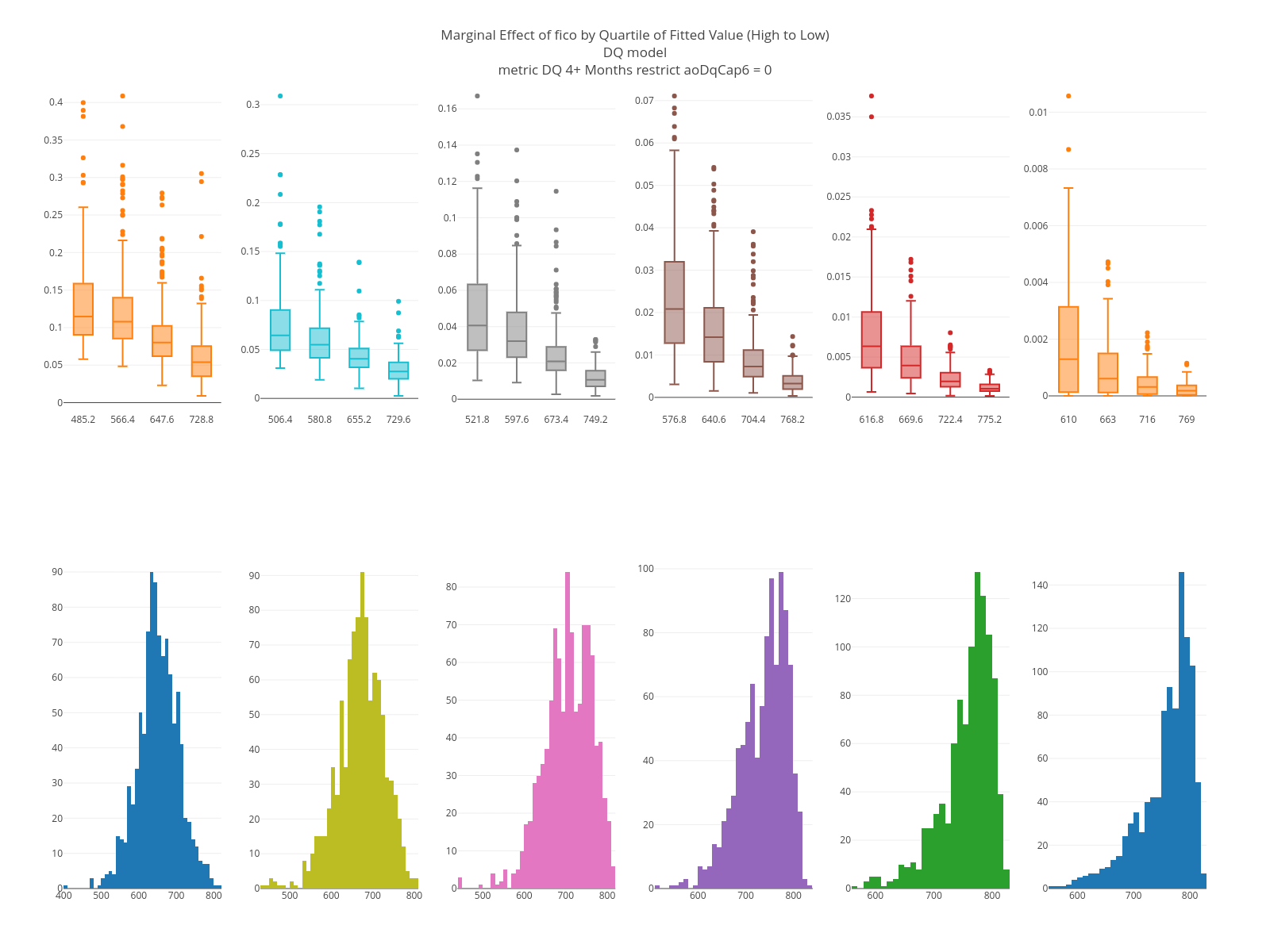
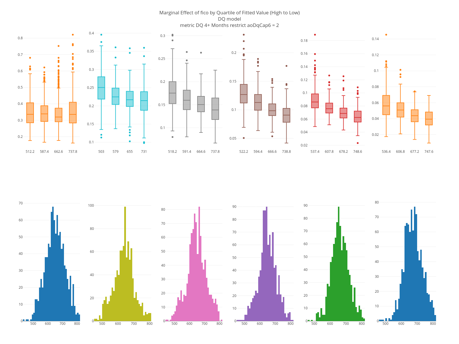
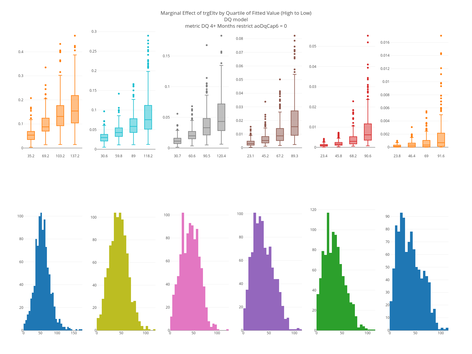
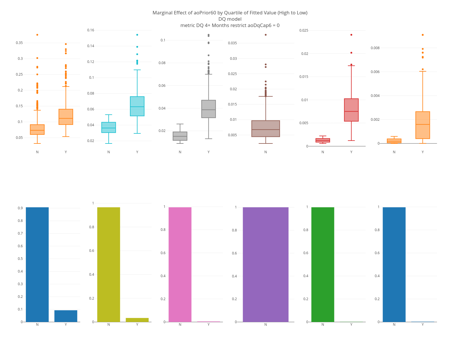
Feature Assessments
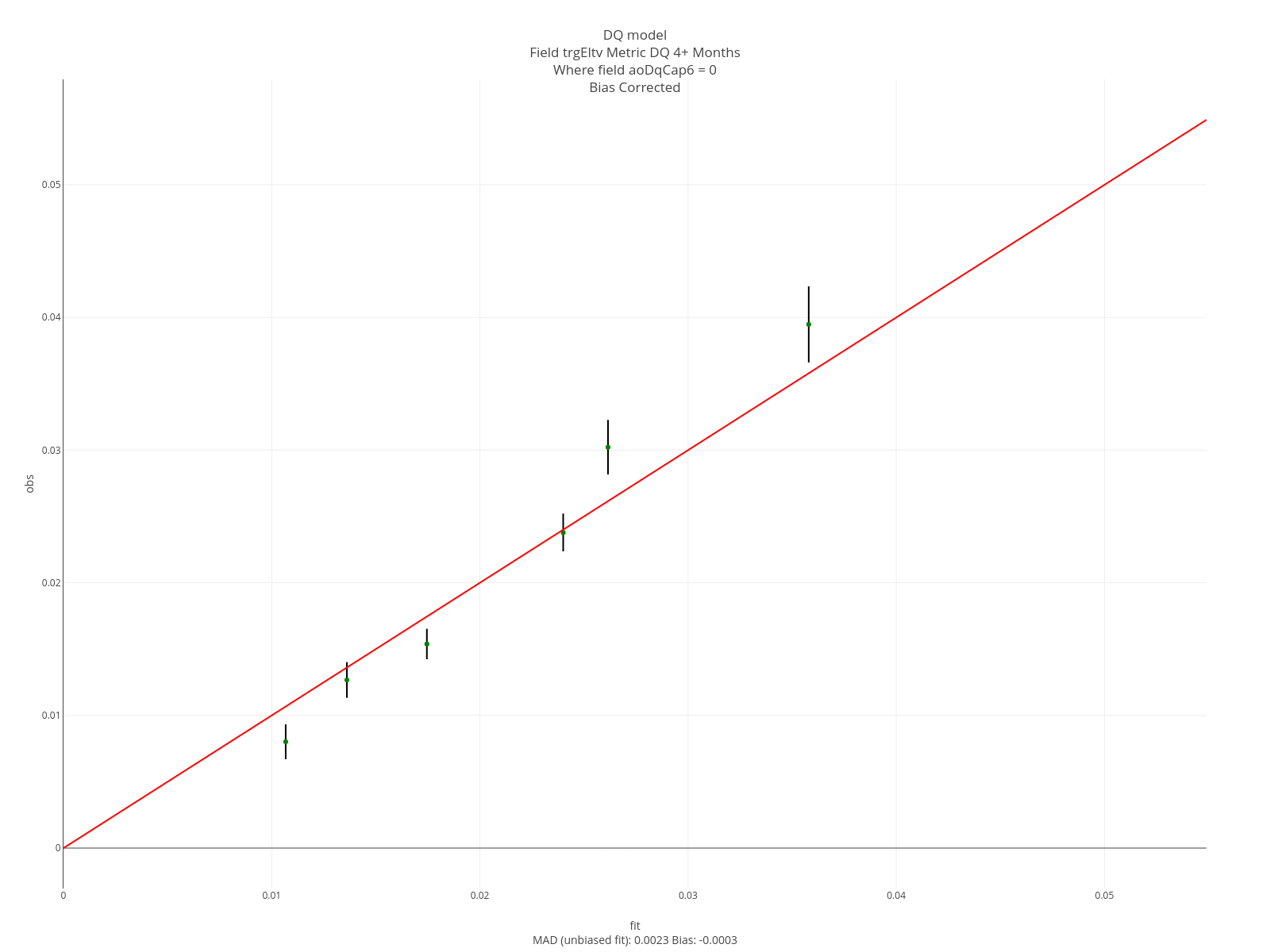
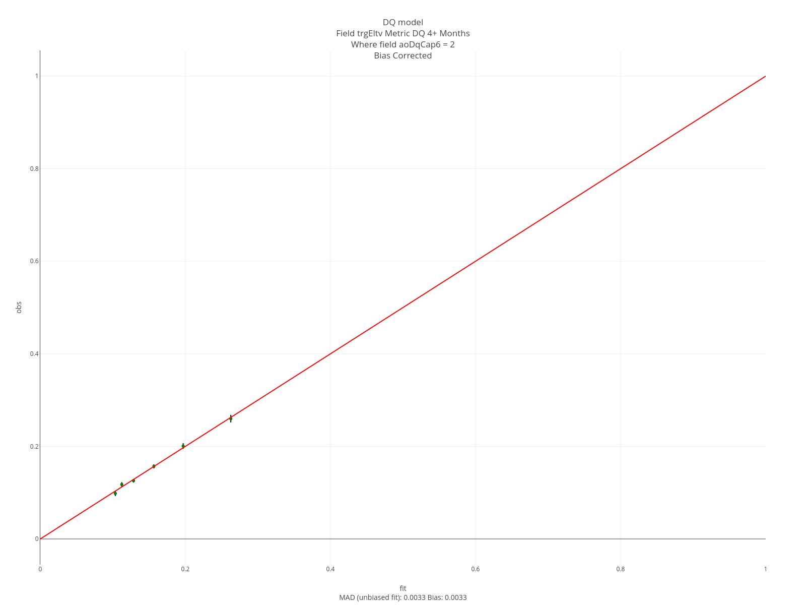
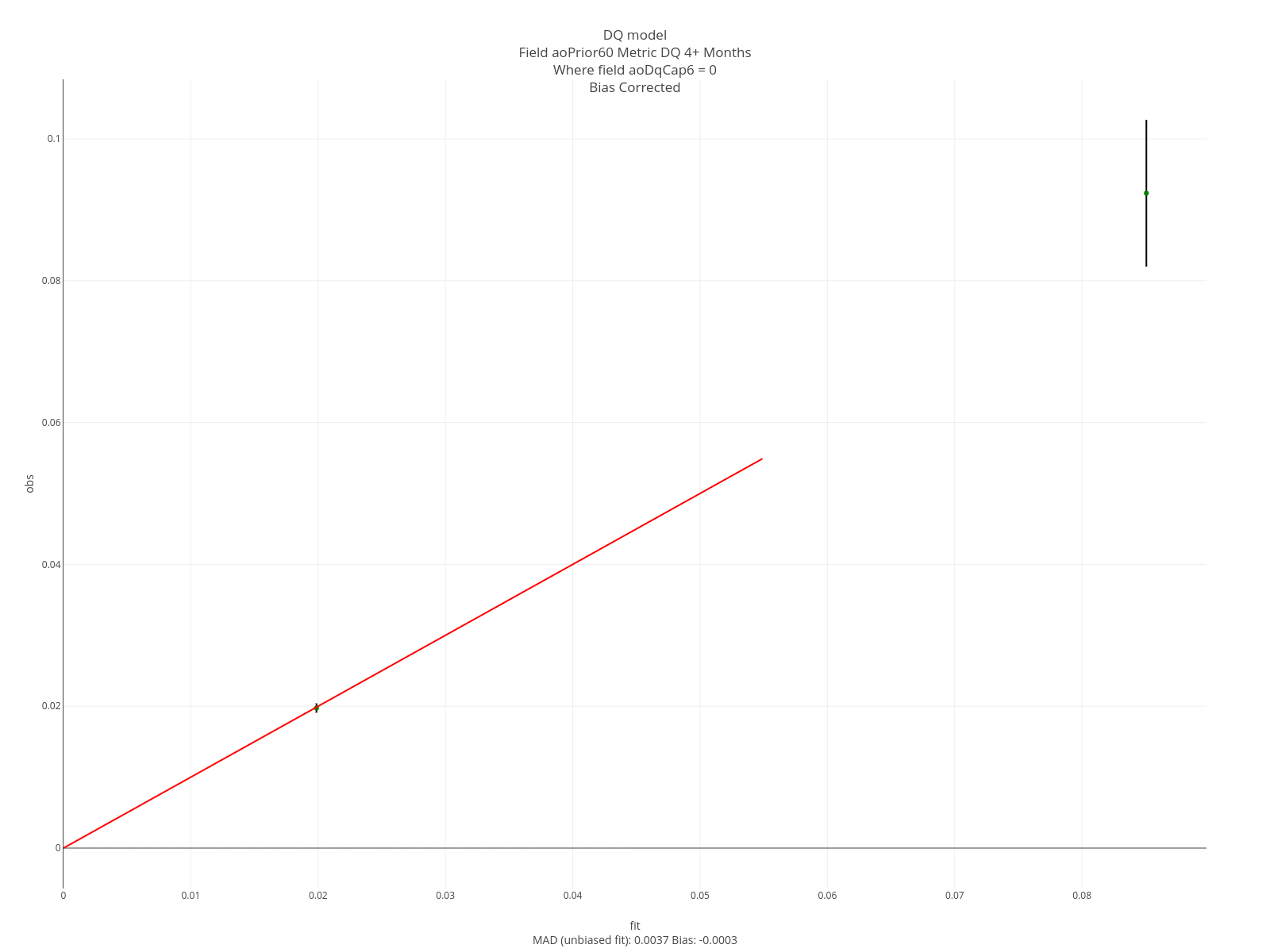
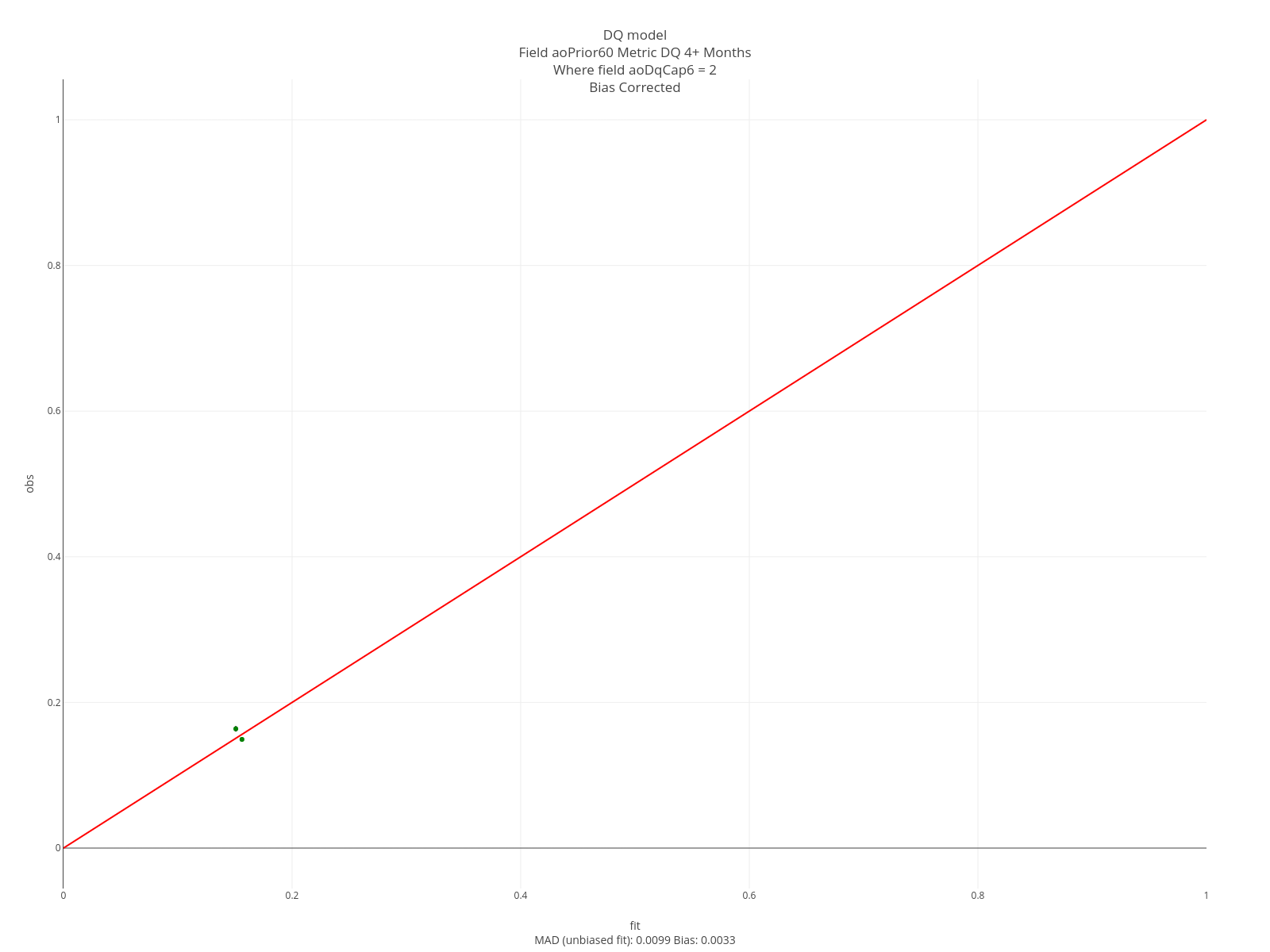
The graphs below are marginal plots. The left column is based on loans that are current at the as-of date; the right columns loans that are 60 days delinquent. FICO has an effect in both sets but is larger for loans that are current. The estimated LTV at the target date is strong in both but having been 60 days delinquent in the past matters only for current loans.


The KS plots are below. Loans that are current are easier to separate than loans that are 60 days down. Note, too, that a “1” in these graphs is based on being 4+ months delinquent on a specific month, which is a harder problem than being 4+ months delinquent in a time window.


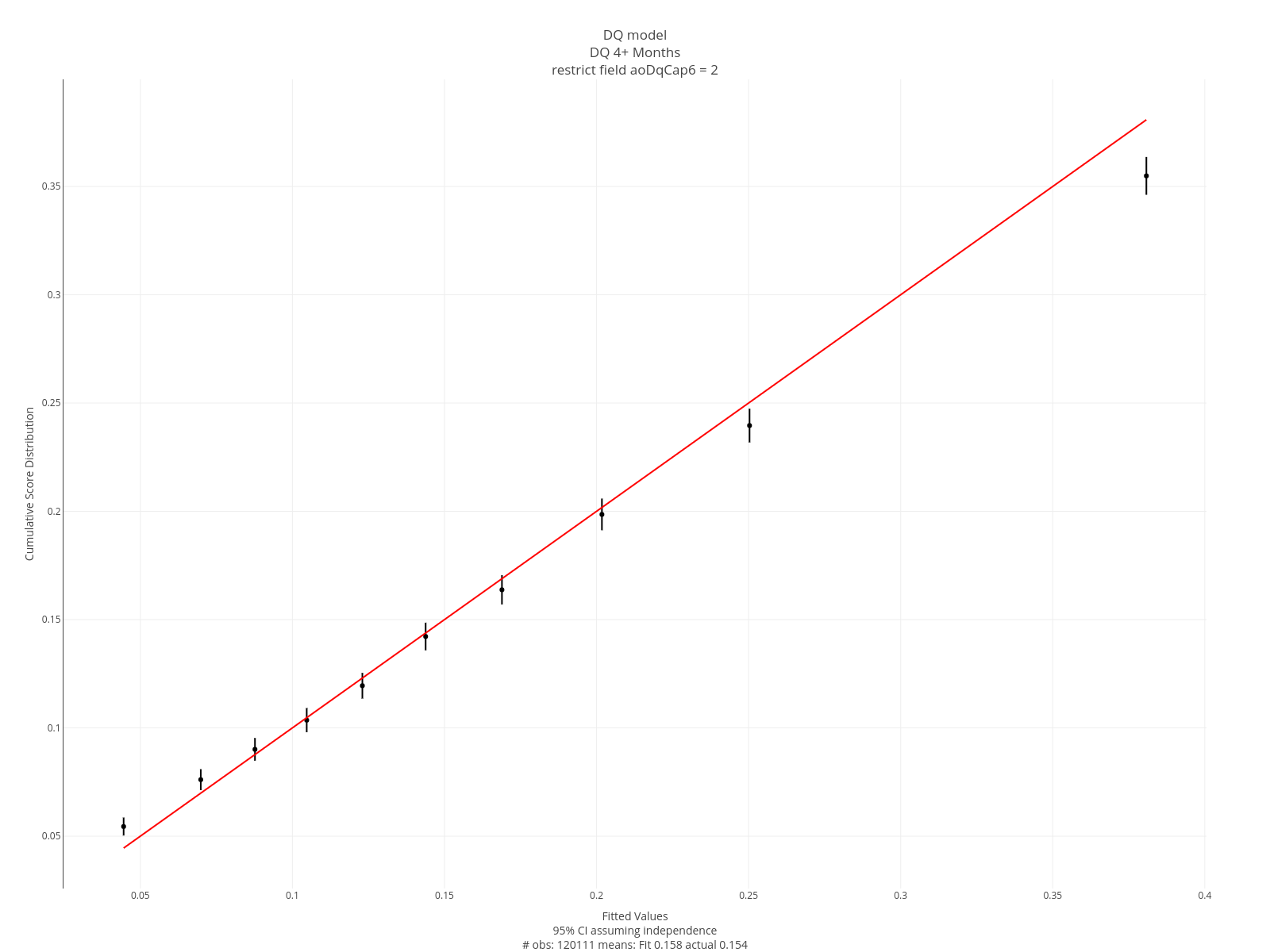
The decile plots are below. The fit is very good.

The segment plots for the same features are below. For current loans, FICO covers a slightly larger range than Eltv but for current loans it works the other way. The intuition is that knowing the borrower is 2 months delinquent on this loan is more relevant than knowing their FICO at some point in the past. Similar intuition applies to knowing they’ve been 2 months delinquent in the past.